Last modification: E. Solano 1 Jul 2014 15:00h
Case I: The Collinder 69 open cluster (Bayo et al., 2008 A&A 492, 277)
Getting started
- Step 1.- Go to http://svo2.cab.inta-csic.es/theory/vosa/
- Step 2.- To use VOSA you need to be registered. Click on "Register" and fill in the fields (email, name and passwd).
- Step 3.- VOSA can be used to study stellar/substellar and extragalactic data. For this use case, click on "Stars and brown dwarfs".
- Step 4.- Cut and paste in a file the list of objects in "VOSA format" included in vosa_substellar.txt
Tag "Files"
- Step 5.- Upload the file in VOSA ("File to upload"). Give a description (free text) and do not forget to select "magnitudes" as file type. Then, click "Upload". The message "your-file-name" has been succesfully uploaded! will appear. Click "Continue".
Tag "VOPhot"
- Step6.- Skip the tag "Objects". With the next tag ("VO Phot.") we can complement our "user photometry" with photometry found in VO services. For this use case, click "unmark All" and select only 2MASS, WISE and CMC-14. Then, click "Query selected services" at the bottom of the page. IMPORTANT!! Do not forget to click on "Save VO photometry" once the results are displayed. Otherwise, you will loose all the information gathered from VO catalogues. Once this is done, a summary table with the VO photometry (in flux units) will appear.
Tag "SED"
- Step7.- This tag gives us the possibility of visualising/modifying the SED before the model fitting. Bad photometric points / upper limits can be deleted / no included in the fitting by cliking on the corresponding check box and click on "Apply changes". If VOSA detects an infrared excess, the photometric points are drawn in black and are not considered in the fitting process. The user can manually overrride it and specify a new limit in the "Excess" panel. Veiling can also be taking into account: Photometric points bluewards than the wavelength included in the "Apply UV/blue excess up to" box will not be included in the fit. For this use case, do not make any change.
Tag "Chi-2 Fit"
- Step8.- In the next tag ("Chi-2 Fit"), different grids of theoretical models covering different ranges of physical parameters are displayed. For this case, click "unmark All" and select only the "BT-Settl". To save time, do not tick "Include model spectrum in fit plots". Finally, click on "Next:Select model params".
- Step9.- In this window, we can refine the range of physical parameters that will be used for the fit. We will make the following assumption:
- Teff: 2000-5000K
- logg: 3.5-5.0
- meta=0.
- Then, click on "Next: Make the fit".
- Step10.- We can now see a summary table with the best fit results. Click on "Show graphs" to have a look at the graphics. The effective temperatures and logg obtained after the fitting are:
- LOri0005: Teff: 3800K logg: 4.0
- LOri0029: Teff: 3200K logg:4.0
- LOri0048: Teff: 3600K logg: 4.0
- LOri0158: Teff: 3200K logg:5.5
- LOri0162: Teff: 2400K logg:3.5
Tag "Bayes Analisis"
- Step11.- Alternatively, you can perform a Bayesian fitting using the "Bayes analysis" tag. To do so, we select the same collection of models and range of physical parameters as in Step9. Then, click "Make the fit". A summary table with information on the model with the highest probability is shown. For each object, the information is graphically displayed by clicking on the object name (top left panel).
- LOri0005: Teff: 3800K (67.42%) logg: 4.0 (68.67%)
- LOri0029: Teff: 3400K (40.44%) logg: 4.0 (86.56%)
- LOri0048: Teff: 3400K (40.78%) logg: 4.0 (54.51%)
- LOri0158: Teff: 3200K (49.93%) logg: 4.0 (49.75%)
- LOri0162: Teff: 2400K (100%) logg: 3.5 (37.93%)
Tag "HR Diag."
- Step12.- In order to estimate ages and masses for our objects we will make use of the "HR Diag." tab. Click on "Make the HR diagram". Ages derived for LOri0005, LOri0048 and LOri0162 are consistent with the age of the cluster (upper limit: 12-16 My).
Tag "Save Results"
- Step13.- You can save different type of results (plots, VO photometry, Bayes fit, chi-2 fit,...) using the "Save Results" tag.
Tag "Log"
- Step14.- A summary of all steps executed to carry out the workflow can be found in the "Log" tag.
Tag "Help"
- Step15.- A detailed description of how VOSA works can be found in the "Help" tag.
Case II: The role of extinction on the physical parameters obtained from the SED fitting.
- Step 1.- Cut and paste in a file the list of objects in "VOSA format" included in vosa_case2a.txt
- Step 2.- Go to the "Files" tag. Upload the file. Include a description (e.g. "vosa_case2a"). Click "Upload". It is irrelevant to select "Fluxes" or "Magnitudes" Click "Continue".
- Step 3.- Go to the "Objects" tag. Click "Search for Obj. Coordinates". Tick on "Sesame" coordinates. Click "Save Obj. Coordinates".
- Step4.- With the tag "VO Phot" we look for photometry in VO services. To save time, we only select the following services (the rest of services do not provide results):
- Infrared: 2MASS, DENIS, WISE
- Optical: Tycho-2, Stromgren, UBV
- Click "Query selected services". IMPORTANT: Do not forget to click on "Save VO photometry" once the results are displayed. Once this is done, a summary table with the VO photometry (in flux units) will appear.
- Step5.- Go to the "Chi-2 Fit" tag. Select "Kurucz". Click on "Next: Select model params". Do not change the parameter range. Then click on "Next:Make the fit".
- Step6.- We can now see a summary table with the best fit results. Click on "Show graphs" to have a look at the graphic. The effective temperatures obtained after the (very good) fitting is Teff: 6250K
- Step7.- Go back to the "Files" tag. Upload the file vosa_usecase2b. Include a description (e.g. "vosa_case2b"). Click "Upload". It is irrelevant to select "Fluxes" or "Magnitudes". Click "Continue"
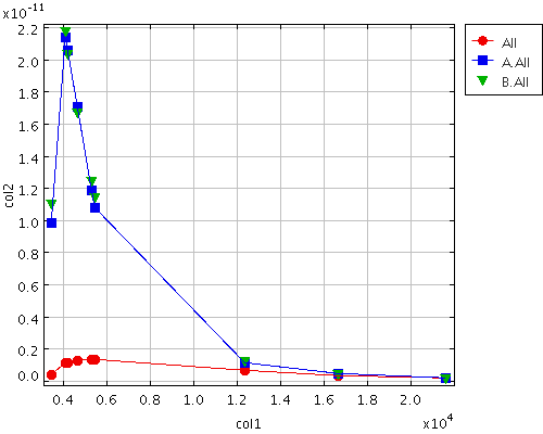
- Step8.- Repeat steps 3-5. Now we get Teff: 33000K with also a very good fit. What is causing the large differences in Teff if we compare these values with those calculated in Step6? The answer is the extinction (in the first case we were assuming no extinction) which has a strong impact on the SED shape. HD302505 is a O9.5III star (SIMBAD) with a E(B-V)=1.15 (Denoyelle 1977A&AS...27..343D).
To have an idea of the importance of extinction, see the figure given below. Red circles represent the observed SED of a star with E(B-V)=0.76. Blue squares represent the SED of the same star after the reddening correction. Forget about the green triangles.